Time-Series Cross-Correlation in Safety Analytics: Proving When Leading Indicators Actually Lead
Physical safety controls do not operate on calendar months; they operate on maintenance repair cycles. When reporting software rolls daily logs into 30-day totals, it erases the timeline that proves whether an inspection actually prevented a failure.


If you roll fifty safety audits and two precursor events into the same monthly spreadsheet row, you erase the timeline that proves whether one prevented the other.
Monthly trend analysis—the method used in the Safety Metrics Screener and the validation framework—evaluates metrics across 12 to 36 months of data. That monthly approach works well for long operational cycles: it proves whether closing corrective actions within 60 days drives down incident rates, or whether a sustained overtime spike serves as a Forewarning signal for worker fatigue.
However, monthly screening has an unavoidable operational blind spot: it cannot see what happens day to day.
If a supervisor spots a defective component on Day 1, an equipment failure occurs on Day 3, and maintenance completes the repair on Day 6, monthly reporting records both the audit and the failure in the exact same 30-day row. The calculation registers them as happening at the exact same time (Lag 0)—hiding the fact that the inspection identified the hazard first.
When a physical barrier operates on a short repair cycle—such as fixing a machine guard or valve within 5 to 14 days—monthly totals wipe out that sequence. Your inspections get dismissed as Concurrent or Weak, even when field verifications are actively protecting the plant.
To audit these short-cycle physical barriers, you need daily time-series analysis that tracks the timeline day by day.
1. Two Operational Timeframes
To build an empirical safety system, you must separate your metrics into two distinct operational tiers:
Why Monthly Totals Hide Physical Controls
A safety check completed at 8:00 AM does not prevent an equipment failure at 8:05 AM. It identifies a cracked mounting bracket on a conveyor drive guard.
The hazard is not eliminated when the inspector hits submit on their tablet. It is eliminated five days later, when maintenance fabricates a replacement bracket, locks out the conveyor drive, and bolts the steel mesh into place.
Physical safety controls operate on a delay: the time it takes maintenance to complete a repair (Mean Time to Repair, or MTTR). When reporting software rolls daily records into monthly totals, that sequence disappears.
If a vibration spike shears the cracked bracket two days later—before maintenance arrives—the monthly spreadsheet records both the inspection and the breakdown in the exact same row. The calculation treats them as happening at the same time (Lag 0). It wipes out the timeline and hides the fact that the inspection caught the defect first, inside an open maintenance gap. Conversely, when maintenance completes the repair on time, the monthly total rolls the audit together with unrelated end-of-month events, burying the five-day window where the barrier protected the line.
This analysis does not make you responsible for maintenance repair backlogs. It gives you the data to show plant and maintenance managers exactly how open work orders leave physical barriers compromised. What reliability engineers measure as repair turnaround is what safety systems experience as barrier latency; when you connect the two, safety data translates directly into plant maintenance schedules instead of competing with them.
Separate Critical Barriers from Routine Housekeeping
Daily time-series analysis will fail if you treat every inspection as equal. Signing off on fifty eyewash station tags has zero physical connection to preventing a conveyor nip-point injury or a pipe blowout.
Before running any calculations, you must separate critical barrier audits (verifications of machine guards, pressure relief valves, interlocks, and lockout/tagout) from routine facility housekeeping.
Here is why: a site might log forty housekeeping walk-throughs and two machine guard checks in a single shift. Housekeeping volume fluctuates randomly day to day (whether supervisors logged 35 or 48 tags), introducing large daily swings into the total count. Because eyewash checks have zero physical connection to machine breakdowns, adding that high-volume paperwork dominates the calculation. It drives the correlation coefficient down to zero, falsely convincing leadership that field inspections have no protective effect. Always filter your inspection database by barrier category before running the analysis.
2. Three Practical Statistical Concepts
Auditing daily operational records requires three concepts: stationarity, cross-correlation, and predictive precedence.
Concept 1: Stationarity (Removing Operational Drift)
Industrial activity fluctuates across the operational calendar: planned overhauls, seasonal production surges, and weather constraints continuously shift baseline activity.
During a major plant turnaround, worked hours double, contractor headcounts surge, and daily inspections multiply fivefold. Because thousands of high-risk tasks are underway at once, minor equipment strikes and near-misses naturally rise.
If you compare raw daily inspection counts directly against incident counts, both lines rise and fall simply because the plant is busier. The calculation will show a strong correlation, but it is completely false: both metrics are merely mirroring plant workload.
To eliminate this distortion, make the data stationary. In plain terms: instead of asking "how many inspections did the site log today?", ask: "did the site complete more or fewer inspections today compared to yesterday?"
Calculating day-over-day changes—subtracting yesterday's total from today's (known as differencing)—removes seasonal shifts and overall production volume. What remains is the real daily movement: sudden spikes or drops in barrier verification.
What to Track When Injuries Are Rare
In a well-run facility, recordable injuries and lost-time events are rare—often fewer than five or ten a year. If you try to calculate day-over-day changes on a daily incident log where 98% of the rows are zero, the math breaks down. When almost every day shows zero change, the calculation has no variation to measure.
Do not force time-series math onto a column full of zeros. Track operational precursors instead:
- Machine & Conveyor Safety: Emergency-stop pull-cord trips, light-curtain interruptions, or interlock faults.
- Hazardous Energy (LOTO): Maintenance jobs stopped during pre-task checks because energy isolation was incomplete or stored pressure was found.
- Mobile Equipment: Forklift impact sensor alerts, speed-zone breaches, or pedestrian proximity sensor alarms.
- Process Operations: Emergency shutdown (ESD) trips, safety bypasses logged in the control room, or flange leaks during startup.
Choose precursors that measure whether physical barriers are holding, not minor clutter. Logging twenty misplaced pallets or untied bootlaces will never predict a severe injury. Operational precursor events occur frequently enough across a facility to provide a usable daily count, while directly tracking the physical breakdown of your barriers.
Concept 2: Cross-Correlation (Shifting the Timeline)
Standard correlation compares two numbers on the exact same day: audits completed today against incidents occurring today.
Cross-correlation shifts the inspection column forward against your precursor events, day by day, across a defined window—typically 21 days (three operational weeks), which matches the standard lifecycle of a plant maintenance work order:
- Lag 0 days: Did today's barrier checks correlate with today's precursor events?
- Lag 1 day: Did today's barrier checks correlate with tomorrow's precursor events?
- Lag 7 days: Did today's barrier checks correlate with precursor events one week later?
In statistical software and the Safety Metrics Screener, each forward step is called a lag day:
- Leading: When barrier checks go up, precursor incidents drop 5 to 12 days later (negative correlation). This confirms a true operational lead time: your team is finding worn parts or bypassed interlocks and correcting them before an incident occurs.
- Forewarning: When an activity increases, future incidents also increase (positive correlation). This tracks accumulating operational risk—for example, consecutive overtime shifts predicting fatigue-related errors 7 days later.
- Concurrent: The relationship only appears on the exact same day (Lag 0) and disappears on future days. On a plant floor, this usually reveals a reactive metric: supervisors only log inspections after an alarm trips or an event occurs.
- Weak: The correlation line stays close to zero across the entire 21-day window, remaining within the band of pure chance. The metric has no measurable preventive effect; it is administrative paperwork.
You do not need IT permission to change corporate software. Export a year of daily logs into a spreadsheet and run the script below (Section 4) on your computer. Once the script shows your site's lag time (for example, 8 days), hand that number to whoever builds your reports.
In Excel or Power BI, they simply line up today's date with the inspections logged 8 days ago. What does that look like on screen? If the team missed three conveyor checks 8 days ago, the dashboard flags an alert today. It tells the crew that uninspected equipment is running right now—giving them a chance to verify the barrier before the shift starts, rather than investigating an incident after it breaks.
Concept 3: Granger Testing (Checking Which Comes First)
Even a lagged correlation does not prove that inspections directly prevented an incident. A third factor—like a meticulous maintenance lead—might be driving up barrier checks while also replacing worn parts ahead of schedule.
To test whether your inspection numbers provide real forecasting value, use a statistical test called Granger causality. Despite the word "causality," it does not prove physical cause and effect. It answers one practical question:
If I forecast next week's precursor events using only past incident history, does adding my daily barrier inspection history make that forecast noticeably more accurate?
If adding your inspection logs clearly reduces forecasting errors (with less than a 5% chance that the improvement was an accident), your inspection data provides real foresight that past incident logs alone cannot give you.
Two Plant Realities to Keep in Mind: First, this test proves timing, not absolute cause. It confirms that inspections consistently happen before incidents drop, but you still need to check for plant conditions: daily worked hours, production throughput, and planned maintenance shutdowns.
Second, safety logs often show zero events for days at a time. They do not flow in smooth, continuous streams like motor temperature or line speed. While data science teams use specialized models for zero-heavy counts, calculating day-over-day changes gives you solid practical evidence that a protective lead time exists—long before you ever need to ask for custom data engineering.
3. How to Classify Your Safety Metrics
When you combine the monthly Safety Metrics Screener with daily time-series testing, every metric on your scorecard falls into one of five operational profiles:
| Metric Profile | How It Behaves (Monthly & Daily) | What Is Happening on Site | What to Do With It |
|---|---|---|---|
| Macro Leading | Negative correlation at 1–3 months in the monthly Screener. | Broad management programs. Long-term risk reduction (for example, closing safety work orders within 60 days). | Keep on Executive Dashboards: Track monthly. Ensure hazard closure times stay on schedule. |
| Micro Leading | Shows as Concurrent in the monthly Screener, but negative correlation at 5–14 days in daily data. | Fast physical barrier control. Shift inspections catch defects that maintenance fixes within routine repair cycles. | Schedule by Protection Window: Set inspection frequency to match the repair cycle (such as re-inspecting critical barriers every 8 days). |
| Forewarning | Positive correlation at future lags in monthly or daily analysis. | Accumulating risk. Tracks operational overload (such as consecutive overtime shifts or mounting repair backlogs). | Use as an Operational Brake: Treat as a warning signal, not a success metric. When it spikes, pause non-routine tasks. |
| Concurrent (Reactive) | Peaks at Lag 0 in both monthly and daily tests. | Post-incident response. Inspections surge only after an alarm sounds or an incident occurs. | Reclassify: Move off the leading indicator scorecard. Track it under incident investigations. |
| Weak | No correlation in either monthly or daily tests. | Paperwork compliance. Forms filled out to meet administrative quotas without touching physical hazards. | Retire: Stop tracking it. Return that time to supervisors to spend in the field. |
4. Run the Analysis Locally (Python Script)
You can copy and run the Python script below on your computer using standard, free data libraries (pandas, numpy, statsmodels).
How to Prepare Your Plant Data
To test your own facility, you need a daily spreadsheet with three columns: Date, barrier_checks, and precursor_events.
1. Match the Check to the Hazard
Never compare total facility inspections against total accidents. The math only works when the inspection checks the exact physical barrier that prevents the incident:
| Hazard Area | What to Count in barrier_checks | Matching Precursor in precursor_events |
|---|---|---|
| Conveyors & Machinery | Machine guard & emergency-stop pull-cord checks | E-stop activations, interlock trip alarms, nip-point jams |
| Forklifts & Vehicles | Daily pre-shift brake and steering checklist tags | Impact sensor alarms, automated speed-zone warnings |
| Hazardous Energy (LOTO) | Lockout/tagout field checks before maintenance | Work halted due to unexpected stored pressure or live power |
2. Three Rules for Your Spreadsheet
- Keep Every Calendar Day: Your spreadsheet must include all 365 days. If the plant was closed on Sunday and zero checks were logged, do not delete the row—enter
0. Skipping weekends breaks the calendar timeline and distorts your actual lead time. - Use Zeros, Not Blank Cells: If no checks were completed or no alarms tripped, enter
0. An empty cell breaks formulas and causes software to drop the day entirely. - Track One Hazard at a Time: Filter your safety software by equipment category before creating daily totals. Never combine forklift inspections and conveyor checks into a single combined number.
Save your spreadsheet as daily_safety_records.csv in the same folder as the script:
Date,barrier_checks,precursor_events
2025-01-01,12,0
2025-01-02,15,1
2025-01-03,14,0
2025-01-04,0,0
2025-01-05,0,0
If you don't have a CSV file yet, the script automatically runs in demo mode—simulating a plant with an 8-day maintenance repair lag—so you can see the math uncover the lead time before plugging in your own records.
The script removes seasonal drift by comparing each day to the day before, plots all 21 future days to reveal your peak lead time, and tests whether inspections reliably happen before incident drops.
import warnings
warnings.filterwarnings("ignore", category=FutureWarning)

import numpy as np
import pandas as pd
import matplotlib.pyplot as plt
from statsmodels.tsa.stattools import adfuller, ccf, grangercausalitytests

# ---------------------------------------------------------
# 1. LOAD YOUR PLANT DATA (OR RUN DEMO)
# ---------------------------------------------------------
# Expected CSV format:
# Date,barrier_checks,precursor_events
# 2025-01-01,12,0
# 2025-01-02,15,1

CSV_FILE = "daily_safety_records.csv"
BARRIER_COL = "barrier_checks"       # Name of your daily barrier check column
PRECURSOR_COL = "precursor_events"   # Name of your daily precursor/event column

try:
    df = pd.read_csv(CSV_FILE, parse_dates=["Date"], index_col="Date")
    df = df[[BARRIER_COL, PRECURSOR_COL]].dropna()
    df.columns = ["barrier_checks", "precursor_events"]
    print(f"Loaded {len(df)} days of plant data from '{CSV_FILE}'.")
except FileNotFoundError:
    print(f"'{CSV_FILE}' not found. Generating 365 days of demo plant data...")
    np.random.seed(42)
    days = 365
    date_index = pd.date_range(start="2025-01-01", periods=days, freq="D")

    # Seasonal operational tempo (e.g., annual overhaul or seasonal production surge)
    operational_tempo = 5 * np.sin(2 * np.pi * np.arange(days) / 365) + 15

    barrier_checks = np.zeros(days)
    precursor_events = np.zeros(days)

    # Simulate daily interactions with an underlying 8-day repair turnaround
    for t in range(days):
        base_risk = 0.12 * operational_tempo[t]
        protective_effect = 0.09 * barrier_checks[t - 8] if t >= 8 else 0.4
        lam_p = max(0.05, base_risk - protective_effect + np.random.uniform(0.1, 0.3))
        precursor_events[t] = np.random.poisson(lam=lam_p)

        reactive_bump = 3.0 * (precursor_events[t - 1] + precursor_events[t - 2]) if t >= 2 else 0.0
        lam_a = operational_tempo[t] + reactive_bump
        barrier_checks[t] = np.random.poisson(lam=lam_a)

    df = pd.DataFrame({
        "barrier_checks": barrier_checks,
        "precursor_events": precursor_events
    }, index=date_index)

# ---------------------------------------------------------
# 2. STATIONARITY TESTING & UNIFIED DIFFERENCING
# ---------------------------------------------------------
print("--- Step 1: Testing Stationarity (ADF Test) ---")
barrier_adf = adfuller(df["barrier_checks"].dropna())
precursor_adf = adfuller(df["precursor_events"].dropna())

print(f"[Barrier Checks]    ADF Statistic: {barrier_adf[0]:.4f} | p-value: {barrier_adf[1]:.4f}")
print(f"[Precursor Events]  ADF Statistic: {precursor_adf[0]:.4f} | p-value: {precursor_adf[1]:.4f}")

# Econometric rule: If either series has seasonal drift, difference both so both series are stationary
needs_differencing = (barrier_adf[1] > 0.05) or (precursor_adf[1] > 0.05)

if needs_differencing:
    print("  --> Non-stationarity detected. Applying day-over-day differencing to both series.")
    clean_df = pd.DataFrame({
        "barrier_diff": df["barrier_checks"].diff(),
        "precursor_diff": df["precursor_events"].diff()
    }).dropna()
else:
    print("  --> Both series are stationary. Retaining raw counts.")
    clean_df = pd.DataFrame({
        "barrier_diff": df["barrier_checks"],
        "precursor_diff": df["precursor_events"]
    }).dropna()

# ---------------------------------------------------------
# 3. CROSS-CORRELATION FUNCTION (CCF)
# ---------------------------------------------------------
max_lags = 21

# In statsmodels, ccf(x, y)[k] computes correlation between x[t+k] and y[t].
# To test if barrier checks today predict precursor drops k days in the future:
# x is precursor_diff (future outcome) and y is barrier_diff (leading activity).
ccf_values = ccf(clean_df["precursor_diff"], clean_df["barrier_diff"], adjusted=False)[:max_lags]

# Two-tailed 95% confidence interval (chance variation threshold)
conf_interval = 1.96 / np.sqrt(len(clean_df))

print("\n--- Step 2: Forward Cross-Correlation (Barrier Checks[t] vs Precursors[t + k]) ---")
for lag in range(max_lags):
    sig_flag = " [SIGNIFICANT LEADING]" if ccf_values[lag] < -conf_interval else ""
    print(f"Lag +{lag:02d} days: r = {ccf_values[lag]:.4f}{sig_flag}")

# Generate Diagnostic Plot
plt.figure(figsize=(10, 5))
lags = np.arange(max_lags)
plt.stem(lags, ccf_values, basefmt=" ")
plt.axhline(y=conf_interval, color="red", linestyle="--", label="95% Confidence Threshold")
plt.axhline(y=-conf_interval, color="red", linestyle="--")
plt.axhline(y=0, color="black", linewidth=0.8)
plt.title("Cross-Correlation: Critical Barrier Checks vs. Future Precursor Events")
plt.xlabel("Future Lag Window k (Days Ahead)")
plt.ylabel("Cross-Correlation Coefficient (r)")
plt.grid(True, linestyle=":", alpha=0.6)
plt.legend()
plt.tight_layout()
plt.savefig("daily_ccf_plot.png", dpi=300)
print("  --> Diagnostic plot saved to 'daily_ccf_plot.png'.")

# ---------------------------------------------------------
# 4. BIDIRECTIONAL GRANGER CAUSALITY TEST
# ---------------------------------------------------------
print("\n--- Step 3: Granger Causality Assessment (Bidirectional) ---")

def run_granger(data_matrix, maxlag=14):
    results = grangercausalitytests(data_matrix, maxlag=maxlag, verbose=False)
    sig_lags = []
    for lag, metrics in results.items():
        p_val = metrics[0]["params_ftest"][1]
        if p_val < 0.05:
            sig_lags.append((lag, p_val))
    return sig_lags

# Direction 1: Barrier Checks -> Precursors (Testing proactive protection)
# In statsmodels: Column 0 is Effect (Y), Column 1 is Cause (X)
forward_input = clean_df[["precursor_diff", "barrier_diff"]].values
forward_lags = run_granger(forward_input, maxlag=14)

if forward_lags:
    print("Result 1: Barrier Checks hold PREDICTIVE PRECEDENCE (Checks lead Precursors):")
    for lag, p_val in forward_lags:
        print(f"  - Lag +{lag} days (F-test p-value = {p_val:.4f}) | Protective lead verified.")
else:
    print("Result 1: No statistically significant forward causality found.")

# Direction 2: Precursors -> Barrier Checks (Testing post-incident reactive surges)
reverse_input = clean_df[["barrier_diff", "precursor_diff"]].values
reverse_lags = run_granger(reverse_input, maxlag=5)

if reverse_lags:
    print("\nResult 2: Precursor Events trigger a POST-INCIDENT INSPECTION SURGE (Precursors lead Checks):")
    for lag, p_val in reverse_lags:
        print(f"  - Lag +{lag} days (F-test p-value = {p_val:.4f}) | Post-incident inspection surge detected.")
else:
    print("\nResult 2: No reactive inspection surge detected.")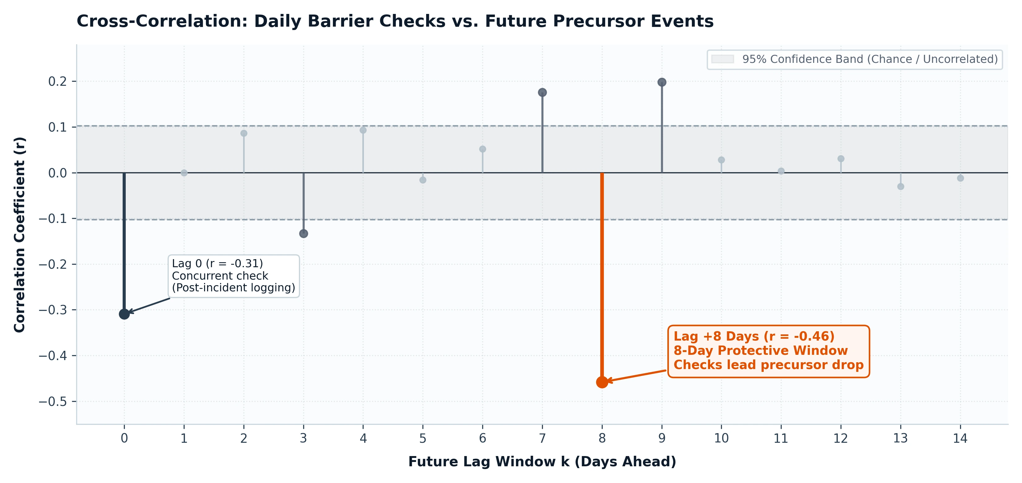
Figure 1: Diagnostic cross-correlation output from the 365-day plant dataset. The downward spike at Lag +8 days breaks through the 95% confidence band (r = -0.46), confirming that daily barrier checks actively lead a reduction in precursor events 8 days later.
5. Three Operational Rules for Plant Leadership
An 8-day lead time changes how you schedule maintenance and manage daily production. Take that number directly to your plant and maintenance managers with three rules:
1. Set Inspection Intervals to Match the 8-Day Window
If barrier checks protect the line for 8 days, inspecting once a month leaves equipment unverified for 22 days every cycle. Align your inspection schedule directly to that 8-day protection window: critical interlocks, e-stops, and machine guards must be re-checked every 8 days.
2. Match Work Order Turnaround to the 8-Day Clock
A broken interlock switch or loose guard cannot sit in a general 30-day maintenance backlog. If a check protects the line for 8 days, but maintenance takes 14 days to close safety work orders, that barrier sits broken or bypassed for nearly a week. Safety checks and maintenance repairs must run on the exact same clock.
3. Audit the Sequence, Not the Operator
When a line trips or an emergency stop activates, do not start by asking what the operator did wrong that morning. Trace the sequence backward through your maintenance work orders (CMMS):
- Was the barrier inspected 8 days ago?
- Did the check log a defect?
- Did the repair work order sit unassigned in the queue?
When you measure time lag instead of monthly totals, safety stops being an administrative compliance score. It becomes part of plant reliability: inspecting a barrier today is a maintenance trigger that keeps the equipment running next week.


